Clinical Outcomes Prediction
Predicting Hypertension Risk
A machine‑learning dashboard for predicting hypertension risk with patient‑level SHAP interpretability.
Overview
This project builds an end‑to‑end clinical risk prediction system using a Random Forest model and SHAP interpretability. The dashboard allows users to:
- Upload or select patient data
- Generate a hypertension risk prediction
- View global feature importance
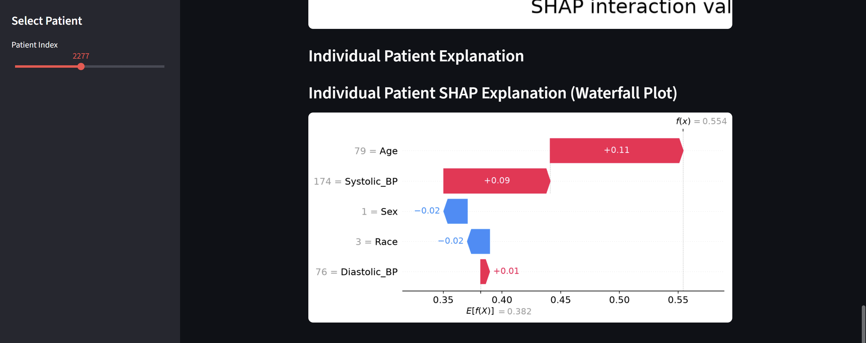
- Explore patient‑specific SHAP explanations
- Interpret model behavior using waterfall and beeswarm plots
The goal is to provide transparent, interpretable clinical ML that supports decision‑making rather than replacing it.
Live Dashboard
You can access the deployed Streamlit app here: Live Streamlit App
GitHub Repository
Goal: Predict Hypertension
1. Basic EDA
- Load the dataset
- print
head() - check for missing values
- look at distributions
- identify target variable
import pandas as pd
import numpy as np
import matplotlib.pyplot as plt
import seaborn as sns

from sklearn.model_selection import train_test_split
from sklearn.preprocessing import StandardScaler
from sklearn.metrics import classification_report, roc_auc_score
from sklearn.linear_model import LogisticRegression
from sklearn.ensemble import RandomForestClassifier

## Load NHANES Data
demo = pd.read_sas("data/DEMO_J.XPT")
bpq = pd.read_sas("data/BPQ_J.XPT")
bpx = pd.read_sas("data/BPX_J.XPT")

## Merge datasets
df = demo.merge(bpq, on="SEQN", how="left")
df = df.merge(bpx, on="SEQN", how="left")

print(df.shape)
df.head()
(9254, 76)
| SEQN | SDDSRVYR | RIDSTATR | RIAGENDR | RIDAGEYR | RIDAGEMN | RIDRETH1 | RIDRETH3 | RIDEXMON | RIDEXAGM | ... | BPAEN1 | BPXSY2 | BPXDI2 | BPAEN2 | BPXSY3 | BPXDI3 | BPAEN3 | BPXSY4 | BPXDI4 | BPAEN4 | |
|---|---|---|---|---|---|---|---|---|---|---|---|---|---|---|---|---|---|---|---|---|---|
| 0 | 93703.0 | 10.0 | 2.0 | 2.0 | 2.0 | NaN | 5.0 | 6.0 | 2.0 | 27.0 | ... | NaN | NaN | NaN | NaN | NaN | NaN | NaN | NaN | NaN | NaN |
| 1 | 93704.0 | 10.0 | 2.0 | 1.0 | 2.0 | NaN | 3.0 | 3.0 | 1.0 | 33.0 | ... | NaN | NaN | NaN | NaN | NaN | NaN | NaN | NaN | NaN | NaN |
| 2 | 93705.0 | 10.0 | 2.0 | 2.0 | 66.0 | NaN | 4.0 | 4.0 | 2.0 | NaN | ... | NaN | NaN | NaN | NaN | 202.0 | 62.0 | 2.0 | 198.0 | 74.0 | 2.0 |
| 3 | 93706.0 | 10.0 | 2.0 | 1.0 | 18.0 | NaN | 5.0 | 6.0 | 2.0 | 222.0 | ... | 2.0 | 114.0 | 70.0 | 2.0 | 108.0 | 76.0 | 2.0 | NaN | NaN | NaN |
| 4 | 93707.0 | 10.0 | 2.0 | 1.0 | 13.0 | NaN | 5.0 | 7.0 | 2.0 | 158.0 | ... | 2.0 | 128.0 | 46.0 | 2.0 | 128.0 | 58.0 | 2.0 | NaN | NaN | NaN |
5 rows × 76 columns
Choosing target variable and relavant features
## Hypertention Outcome Variable

# BPQ020: "Ever told you had high blood pressure?"
# 1 = Yes, 2 = No, 7 = Refused, 9 = Don't know

df['hypertension'] = df['BPQ020'].replace({1: 1, 2: 0}).astype('float')
df = df.dropna(subset=['hypertension'])
df['hypertension'].value_counts(normalize=True)

## Select Features for Model
features = [
    "RIDAGEYR",   # age
    "RIAGENDR",   # sex
    "RIDRETH3",   # race/ethnicity
    "BPXSY1",     # systolic BP
    "BPXDI1"      # diastolic BP
]

df_model = df[features + ['hypertension']].copy()
df_model = df_model.dropna()

# ## Rename columns for clarity
df_model = df_model.rename(columns={
    'RIDAGEYR': 'Age',
    'RIAGENDR': 'Sex',
    'RIDRETH3': 'Race',
    'BPXSY1': 'Systolic_BP',
    'BPXDI1': 'Diastolic_BP'
})

features = ['Age', 'Sex', 'Race', 'Systolic_BP', 'Diastolic_BP']

print(df_model.shape)
df_model.head()
(5169, 6)
| Age | Sex | Race | Systolic_BP | Diastolic_BP | hypertension | |
|---|---|---|---|---|---|---|
| 3 | 18.0 | 1.0 | 6.0 | 112.0 | 74.0 | 0.0 |
| 6 | 75.0 | 2.0 | 4.0 | 120.0 | 66.0 | 1.0 |
| 8 | 56.0 | 1.0 | 6.0 | 108.0 | 68.0 | 0.0 |
| 9 | 18.0 | 1.0 | 1.0 | 112.0 | 68.0 | 0.0 |
| 10 | 67.0 | 1.0 | 3.0 | 104.0 | 70.0 | 0.0 |
Exploring the data
From general knowledge, we can suppose that hypertension diagnosis is correlated with age. To see this, we can create a visual representation of hypertension by age.
with_hypertension = df_model[df_model['hypertension'] == 1]

plt.figure(figsize=(10, 6))
sns.histplot(data=with_hypertension, x='Age', multiple='stack', bins=30)
plt.title('Hypertension Cases by Age')
plt.xlabel('Age')
plt.ylabel('Count')
plt.show()
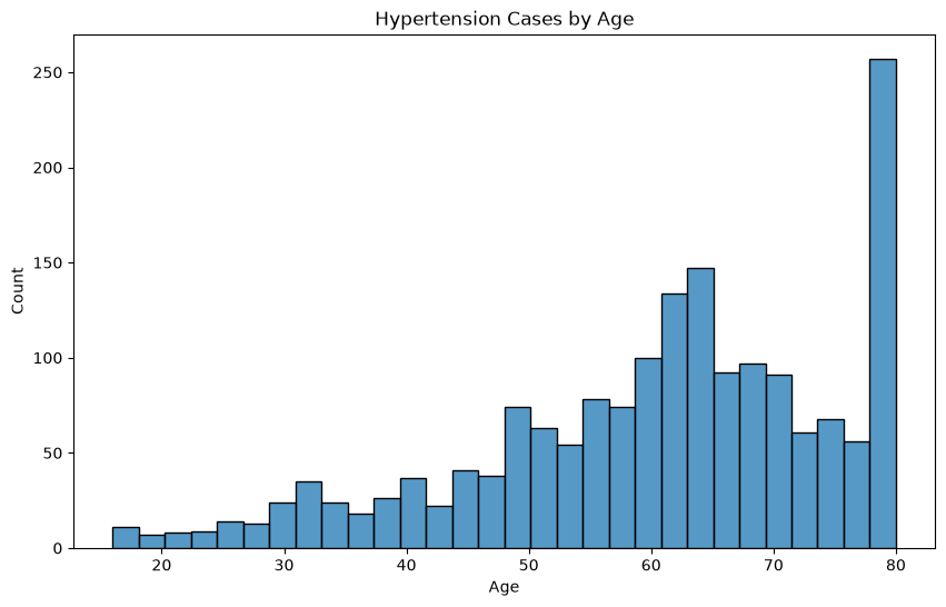
However, this is not necessarily reliable, since there might not have been equal sampling for each age group. Instead, we can look at the ratio of individuals in each age group with a positive hypertension diagnosis.
## Find age range of the samples
print((df_model['Age']).min())
print((df_model['Age']).max())
16.0
80.0
age_bins = [16, 25, 30, 35, 40, 45, 50, 55, 60, 65, 70, 75, 81]
age_labels = [f"{age_bins[i]}-{age_bins[i+1]-1}" for i in range(len(age_bins)-1)]
df_model['Age_Group'] = pd.cut(df_model['Age'], bins=age_bins, labels=age_labels, right=False)

ratio_hypertension_by_age = df_model.groupby('Age_Group')['hypertension'].mean()
plt.figure(figsize=(10, 6))
ratio_hypertension_by_age.plot(kind='bar')
plt.title('Ratio of Hypertension Cases by Age')
plt.xlabel('Age')
plt.ylabel('Ratio of Hypertension Cases')
plt.show()
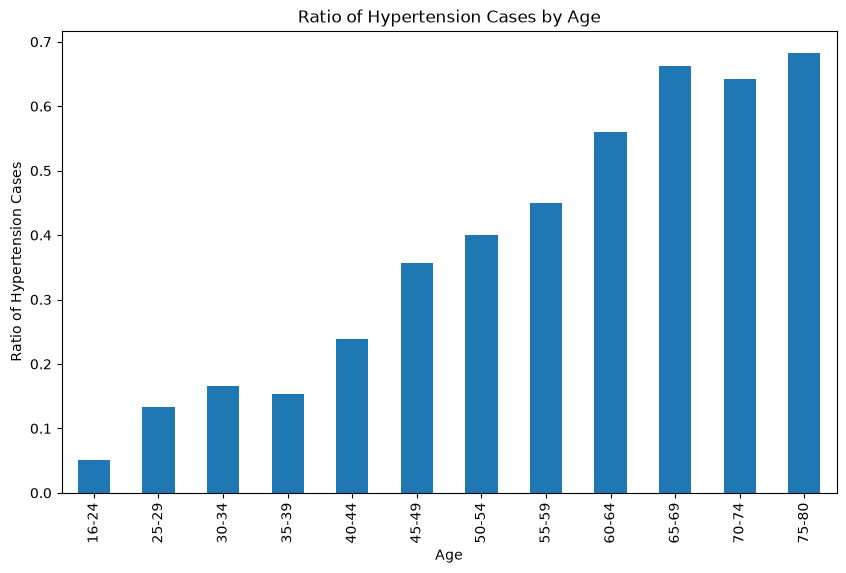
Let’s look at how blood pressure levels relate to hypertension diagnosis.
fig, axes = plt.subplots(nrows=1, ncols=2, figsize=(10, 6))
sns.histplot(data=df_model, x='Systolic_BP', hue='hypertension', multiple='stack', bins=30, ax=axes[0])
axes[0].set_title('Hypertension Cases by Systolic Blood Pressure')
axes[0].set_xlabel('Systolic Blood Pressure')
axes[0].set_ylabel('Count')
sns.histplot(data=df_model, x='Diastolic_BP', hue='hypertension', multiple='stack', bins=30, ax=axes[1])
axes[1].set_title('Hypertension Cases by Diastolic Blood Pressure')
axes[1].set_xlabel('Diastolic Blood Pressure')
axes[1].set_ylabel('Count')
plt.show()
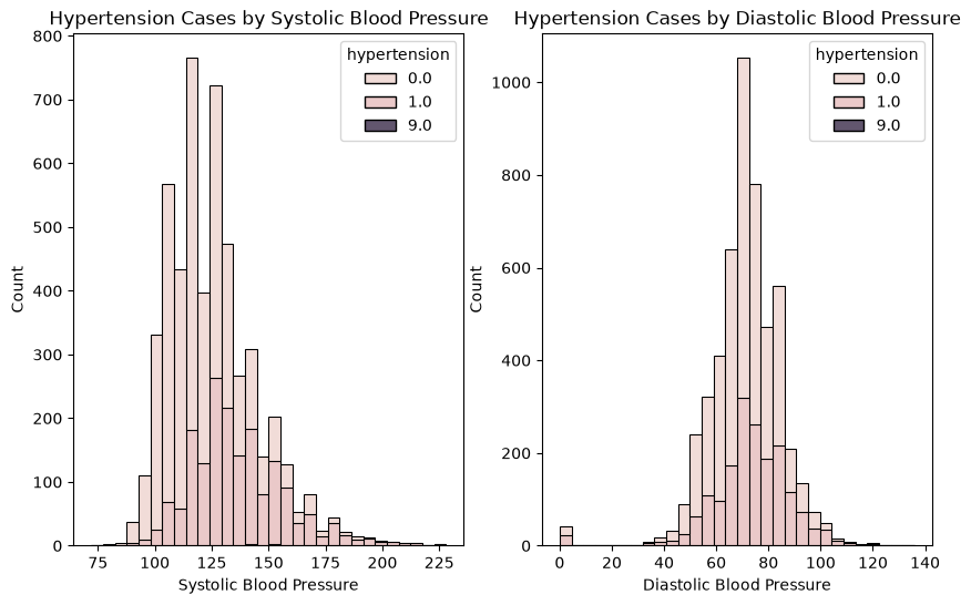
This plot shows us two things.
- The distribution of systolic blood pressure is right-skewed, centered around ~120. The distribution of diastolic blood pressure is approximately a gaussian distribution centered around ~75.
- The ratio of individuals with hypertension increases as systolic and diastolic blood pressure increases.
In other words, “normal” systolic blood pressure is around 120 and diastolic blood pressure is around 75. When these levels increase, an individual is much more likely to have hypertention.
Now that we’ve explored a few variables, let’s look at the correlation between each of the variables using a heatmap.
plt.figure(figsize=(10, 6))
corr = df_model[features + ['hypertension']].corr()
sns.heatmap(corr, annot=True, cmap='coolwarm', fmt=".2f")
plt.title('Correlation Heatmap')
plt.show()
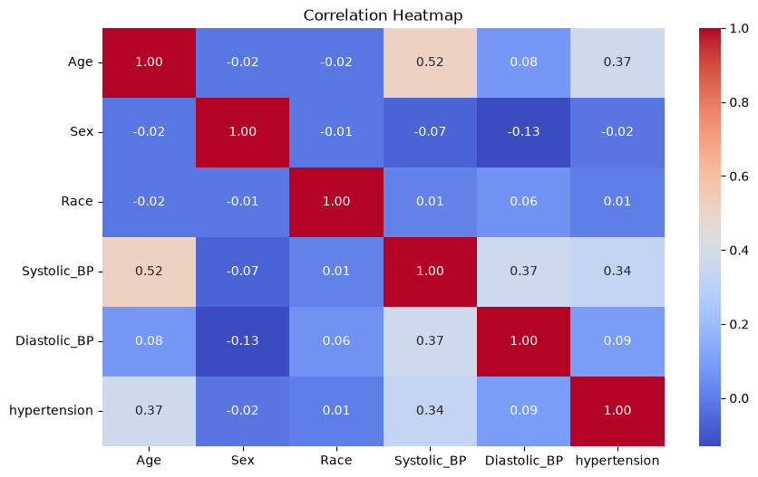
From this heatmap, we can see that age seems to be correlated with systolic blood pressure. The features that are the most correlated with hypertension are age and systolic blood pressure.
2. Predicting Hypertension
## Remove samples with unknown hypertension status
df_model = df_model[df_model["hypertension"].isin([0, 1])]
## Split the data into training and testing sets
X = df_model[['Age', 'Sex', 'Race', 'Systolic_BP', 'Diastolic_BP']]
y = df_model['hypertension']

X_train, X_test, y_train, y_test = train_test_split(
    X, y, test_size=0.2, random_state=42
)

print(X_train.shape, X_test.shape)
(4127, 5) (1032, 5)
# Scale continuous features
scaler = StandardScaler()
X_train_scaled = scaler.fit_transform(X_train)
X_test_scaled = scaler.transform(X_test)
Logistic Regression Model
log_reg = LogisticRegression(max_iter=1000)
log_reg.fit(X_train_scaled, y_train)

y_pred = log_reg.predict(X_test_scaled)
y_prob = log_reg.predict_proba(X_test_scaled)[:, 1]

print("Logistic Regression AUC:", roc_auc_score(y_test, y_prob))
print(classification_report(y_test, y_pred))
Logistic Regression AUC: 0.7886834295537104
              precision    recall  f1-score   support

         0.0       0.75      0.82      0.79       656
         1.0       0.63      0.53      0.58       376

    accuracy                           0.72      1032
   macro avg       0.69      0.68      0.68      1032
weighted avg       0.71      0.72      0.71      1032
Analysis of Results
The AUC result of ~0.789 shows that the model performs well for a baseline model using only a handful of features (optimal results are 0.80-0.90).
Additionally, the results show that the model is better at identifying people without hypertension (precision=0.75, recall=0.82) than with hypertension (precision=0.63, recall=0.53).
Let’s see if using a random forest model yields better results.
Random Forest Model
rf = RandomForestClassifier(
    n_estimators=300,
    max_depth=8,
    random_state=42
)

rf.fit(X_train, y_train)

y_pred_rf = rf.predict(X_test)
y_prob_rf = rf.predict_proba(X_test)[:, 1]

print("Random Forest AUC:", roc_auc_score(y_test, y_prob_rf))
print(classification_report(y_test, y_pred_rf))
Random Forest AUC: 0.7866968571613906
              precision    recall  f1-score   support

         0.0       0.78      0.79      0.78       656
         1.0       0.62      0.61      0.61       376

    accuracy                           0.72      1032
   macro avg       0.70      0.70      0.70      1032
weighted avg       0.72      0.72      0.72      1032
Analysis of Results
This result is similar to the logistic regression model. The AUC result of ~0.787 is good and the model still performs better on predicting the absence of hypertension. The RF model does have slightly better recall on patients with hypertension.
The similarity of the models means that the data is clean and the target and baseline models are correct. It also means that our predictors are mostly linear. This reflects what was seen during the initial EDA.
Please note that the model would likely be improved with more features, including those with non-linear relationships and interactions. For this project I chose to focus on simple features to highlight basic skills and analysis.
Feature Importance (Random Forest)
importances = pd.Series(rf.feature_importances_, index=features)
importances.sort_values().plot(kind="barh", figsize=(8,5))
plt.title("Feature Importance for Hypertension Prediction")
plt.show()
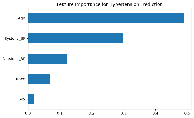
Out of the features I looked at, age had the biggest impact on hypertension prediction. This is consistent with what was hypothesized in the initial EDA.
Save Clean Dataset for Dashboard
df_model.to_csv("nhanes_hypertension_clean.csv", index=False)
3. SHAP Interpretability
import shap

X_test_df = pd.DataFrame(X_test, columns=features)

explainer = shap.Explainer(rf, X_train)
shap_values = explainer(X_test)

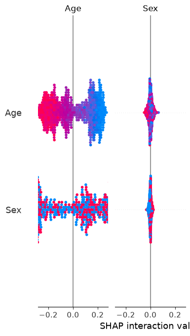
shap.summary_plot(shap_values, X_test_df, plot_type="bar")
Background dataset has 4127 samples but max_samples=100. Subsampling to 100 samples for SHAP value computation. To use all samples, set max_samples=4127 when initializing the masker.
 99%|===================| 2048/2064 [01:27<00:00]
4. Streamlit Dashboard
import pickle

pickle.dump(rf, open("rf_model.pkl", "wb"))
pickle.dump(scaler, open("scaler.pkl", "wb"))