Capstone Project Report
Onset of Type II Diabetes
by Marina Witherell and Vini Karumuru
0 - Table of Contents
1 - Introduction
Type 2 diabetes (T2D) is a significant health issue in the US. In 2022, the CDC reported 10.7% of adults had type 2 diabetes. There are also an estimated 8.5 million undiagnosed cases, and 79 million cases of pre-diabetes with 50% of these cases converting to a lifetime of diabetes. There has been notice of differences of gut microbiome between diabetic and non-diabetic people, which has been observed to have an effect on glucose levels (Stanford Medicine). This project hopes to better understand the changes of the microbiome during diabetic onset and progression. The microbiomes of the nasal samples and those of the fecal samples and the relationship between the two sample types are of prime interest.
The dataset used in this project was taken from the NIH’s Integrated Human Genome Project. Due to limited computational resources, a randomly sampled subset of 1000 samples was taken from the original dataset for our analysis. Our dataset contains samples from 77 pre-diabetic patients. A patient is considered to be pre-diabetic when their fasting blood sugar level is higher than normal but is not high enough to be considered diabetic (this would mean a fasting blood sugar level of 100-125 mg/dL) (Maruthur, 2023). Samples were collected from the patients at two body sites: the feces and the nasal cavity. The dataset contained 465 fecal samples and 535 nasal samples. Most patients had samples taken during more than one timepoint, hence why there are many more samples than there are patients. The microbial DNA was extracted from these samples and underwent 16S amplicon sequencing (Stanford Medicine). As our dataset only contained data from pre-diabetic patients, with no set of control, healthy patients, the focus of our analysis was to compare the fecal and nasal microbiomes of these pre-diabetic patients.
2 - Hypothesis
2.1 Hypothesis 1
The fecal microbiome is more diverse than the nasal microbiome in pre-diabetic patients. This is because the fecal microbiome comes in more direct contact with the internal metabolic processes of the body and therefore is more frequently altered.
2.2 Hypothesis 2
The microbial profile of the skin and fecal samples will be significantly different when using the beta diversity measure. If it is found significant, I will focus on the most abundant taxa and identify the group that explains the differences.
3 - Methods
3.0 Common Methods
We were provided with a phyloseq object created by the Snyder Lab under the iPOP project at Stanford Medicine (Zhou et al, 2019). According to their research paper, the phyloseq object was built using the QIIME pipeline, along with custom scripts in Python and R (Caporaso et al, 2010).The phyloseq object contains sample metadata, the number of reads per sample for each OTU (operational taxonomic unit), and taxonomic information for each OTU.
We began our exploration of the dataset by looking at the number of reads per sample. We summed the number of reads per column in the OTU table and performed calculations with conditional statements on these sums. We found that approximately 3% of our samples (31) contained less than 5,000 reads and the remaining samples (969) contained more than 5,000 reads. The largest sample contained 234,415 and the smallest sample contained 2 reads. The average number of reads per sample was 24,934.
The otu_table in the phyloseq object was normalized using the relative abundance method with the transform_sample_counts() function. The dataset was then split into two separate phyloseq objects, one for each body site (feces and nasal cavity). To accomplish this, we used the subset_samples() function, as the body site information was contained in the sample_data table within the phyloseq object. Most of our methods involved us performing computations and manipulations on these two phyloseq objects separately (but simultaneously), then comparing the two body sites.
3.1 Methods for Hypothesis 1
I tested my hypothesis by employing two measures of alpha diversity: species richness and Shannon index. Species richness was calculated per sample (column in the otu_table) by summing the number of OTUs that had an abundance that was non-zero. Then, as a summary statistic, I determined the median species richness.
I then went on to compute the Shannon index of each sample. The Shannon index (H) is an alpha diversity measure that takes into account both species richness and species evenness. A higher Shannon index would indicate a greater amount of diversity. It can be computed using the equation H=-i=1Spilnpi, where pi is the proportion of the sample’s reads that are found to be the ith OTU, ln is the natural logarithm, and s is the total number of OTUs in the community. The phyloseq package already has an inbuilt function that can calculate various measures of diversity, so I did not have to manually code this calculation. Instead, I utilized the estimate_richness() function with the argument measures = “Shannon”. This gave me a dataframe containing a list of Shannon indexes, one corresponding to each sample. I was then able to plot these indexes at the two body sites as side-by-side boxplots with the ggplot package. I conducted a two-sided Wilcoxon rank-sum test between the two body sites to test the null hypothesis that there is no difference between the median Shannon index of the fecal and nasal microbial communities.
3.2 Methods for Hypothesis 2
Using the normalized data, I conducted a permutational multivariate analysis of variation (PERMANOVA) test on the data. This method compares the variation between the two sample sites to the variation within the two sample sites. I calculated this using the Bray-Curtis distance method, which calculates the similarity of each instance in the phyloseq object. The Bray-Curtis dissimilarity is a measure of beta diversity, showing how different the nasal and fecal microbiomes are from each other. I then went on to identify the most abundant taxa in each body site.
I decided that the best way to do this would be to find the top ten OTUs from the nasal cavity and the top ten from the feces, using the two separate phyloseq objects of data from each body site (in section 3.0). Note that the following steps were done for each of the phyloseq objects separately until stated otherwise. First, I found the row sums of the OTU table and organized the table based on those sums in an increasing to decreasing fashion. Then, I made a function to filter out OTUs that were not present in at least three samples. This was implemented so that an OTU that was highly abundant in only one sample would not make it into the top ten (since it is supposed to represent the most abundant across the body site). From these remaining OTUs, the top ten were subset into a new phyloseq object. I created another filter function that returns the samples that have at least one of the top 10 OTUs present. This was required for the ordination plot. I then updated the phyloseq object to only include those samples, which left me with two filtered phyloseq objects - nasal and feces. I combined these two objects into one and created an ordination plot of the taxa (based on order) and the samples. I also wanted to inspect the top 10% of the OTUs and how that compared to just the top ten from each body site, so I repeated all of the steps above using the top 60 OTUs. This left me with four ordination plots. I also performed another PERMANOVA test on these to find if the top results were significantly different, or if the most abundant from each site were similar.
3.3 Methods for Further Exploration of Top Taxa
To further expand our analysis, I decided that it might be interesting to dive deeper into the top 20 OTUs we had identified to be the most abundant in each body site. More specifically, I wanted to see if there were any trends in the abundances of these top taxa among many patients. I began by removing any patients that did not have samples taken from both body sites. 65 patients remained after doing so. Then, because the dataset contained multiple samples per patient, I averaged each patient’s reads at each body site. For each of the top 10 fecal OTUs, I conducted a one-sided paired Wilcoxon rank-sum test where the mean abundance of this OTU in each patient’s feces was paired with the mean abundance of this OTU at their nasal cavity. I was testing the null hypothesis that the median abundance of the OTU in the feces is either less than or no different from the median abundance of the OTU in the nasal cavity. I repeated this process for the top 10 nasal OTUs (but flipping the body sites in the null hypothesis, to test whether the abundance of these nasal OTUs was significantly greater in the nasal cavity compared to the feces). For any of these one-sided rank-sum tests that resulted in a non-significant p-value (p > 0.05), I conducted a paired two-sided rank-sum test to see if there was any difference between the body sites. The ggpaired() function within the ggpubr package was utilized to plot paired boxplots for each of the top 20 taxa. For the purpose of better visualization, I log-scaled the mean abundance so that more of the data points would be discernible. I used the plot_list() function within the cowplot package to combine multiple of the individual OTU plots into a single figure so that these plots could be more easily compared to one another.
4 - Results
4.1 Results for Hypothesis 1
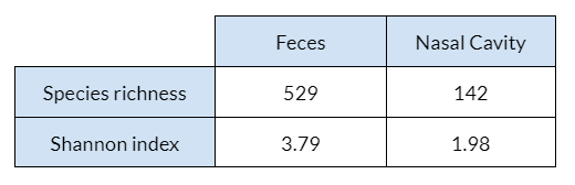
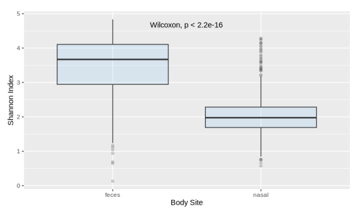
The fecal samples had higher alpha diversity values overall. This is supported by the fact that the median species richness in the fecal samples is more than twice the species richness in the nasal samples (Figure 4.1.1), meaning each sample tended to have a greater number of OTUs detected. Additionally, the fecal samples had a set of significantly higher Shannon indexes when compared to the nasal samples (p < 2.2e-16), which is indicative of greater diversity.
4.2 Results for Hypothesis 2
From the permuted data using the Bray-Curtis dissimilarity, there was convincing evidence that the microbial makeup of the nasal and fecal body sites is significantly different (p-value 0.001). In other words, the beta diversity showed that there are significant differences between the microbiome of the nasal cavity and of fecal matter. This is further illustrated in Figure 4.2.1. When focusing on the top twenty OTUs, the ones from the nasal cavity are more diverse than the ones from feces (Figure 4.2.1 A). However, the two sites do have one taxa in common, Clostridiales. The samples themselves seem to be extremely similar in opposite ways, depending on sample body site (Figure 4.2.1 B). In other words, there is little similarity between groups, but the samples within each group are similar. The results are slightly different when analyzing the top 10% of the OTUs (the sixty most abundant). The nasal taxa are dispersed over a much larger range, while the fecal taxa are condensed in a small area (Figure 4.2.1 C). Additionally, there are some taxa shared between the two body sites, but the nasal cavity displays more diversity. The samples of the top sixty OTUs highlights a similar pattern, with more similarity in the feces microbiome and more variation in the nasal microbiome (Figure 4.2.1 D). It should be noted that the two groups are still noticeably separate.
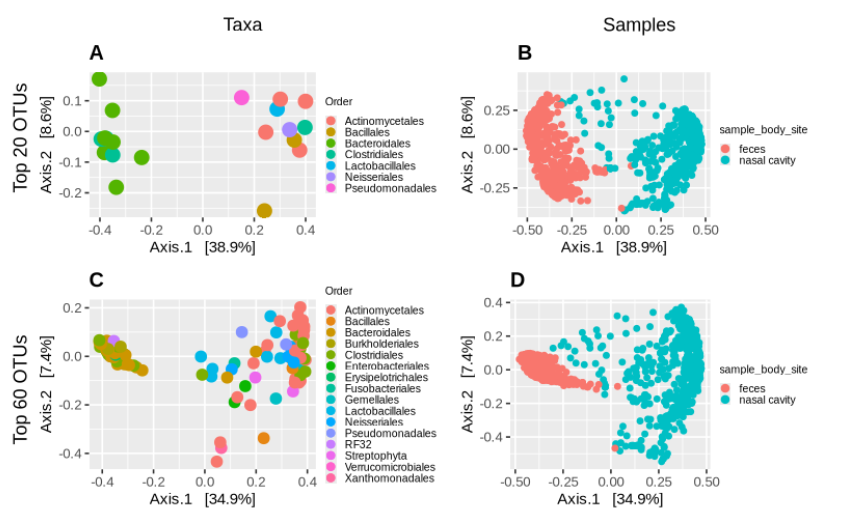
The PERMANOVA test of the top twenty OTUs resulted in a p-value of 0.013, meaning that the most abundant taxa are still significantly different between the groups (despite having one in common). The test of the top ten percent (60) OTUs resulted in a p-value of 0.001, which is even more significant. This pattern suggests that the microbiomes of the nasal cavity and of feces are significantly different, but get progressively more distinct as more samples are taken into account.
4.3 Results for Further Exploration of Top Taxa
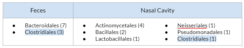
The top taxa in the feces were primarily of the Order Bacteroidales, with a few having the Order Clostridiales. The top taxa in the nasal cavity had a wider range of Orders (6 in total), with the most frequent Order being Actinomycetales. While Clostridiales is represented in both the top taxa of the feces and nasal cavity, the one Clostridiales OTU in this table was not the same OTU as any of the 3 fecal OTUs. Its Family (Tissierellaceae) differs from the Family of the fecal Clostridiales bacteria (Ruminococcaceae).
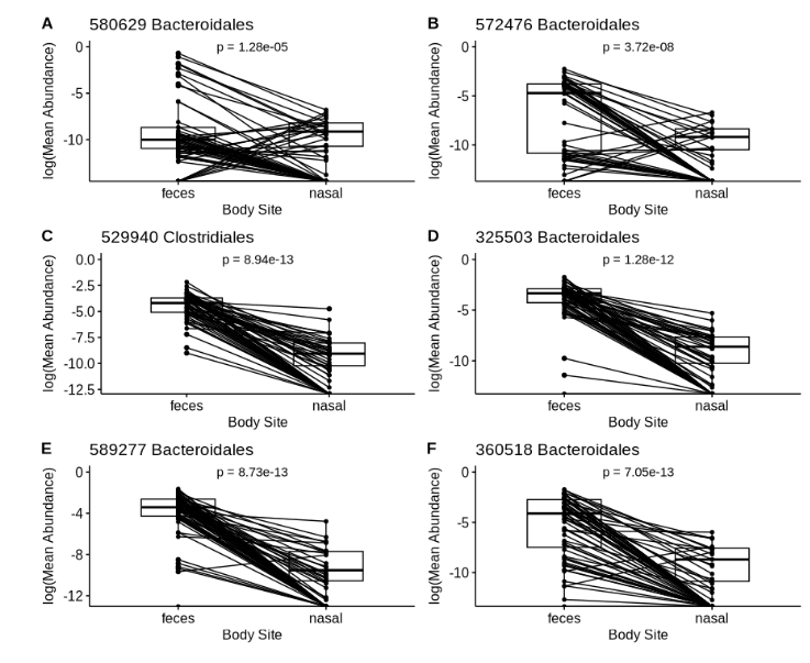
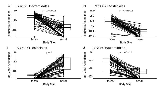
There is no major trend observed in the abundance of these top 10 fecal OTUs at the two body sites. However, 9 out of these 10 top taxa have significantly greater abundance in the feces than in the nasal cavity (p « 0.05). The one exception to this is shown in Figure 4.3.2.I (530327 Clostridales), in which the abundance of this taxa appears to be greater in the nasal cavity than in the feces. For this reason, its one sided p-value is 1 (when rounded). This is unexpected, as we would expect for all of these top 10 taxa (having pinpointed them for their high abundance in the feces) to have greater abundance in the feces in comparison to the nasal cavity. When a two-sided paired Wilcoxon rank-sum test was performed for this OTU, a statistically significant difference was found between the two groups (p « 0.05), indicating that the abundance of this OTU is significantly greater in the nasal cavity.
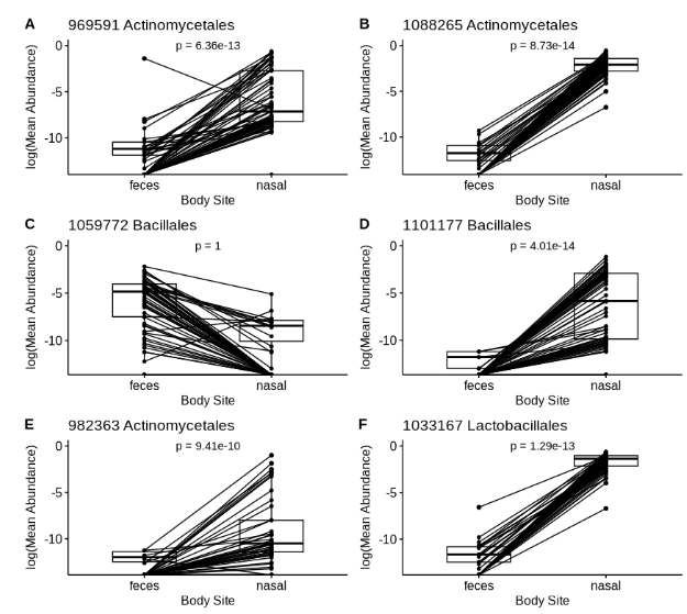
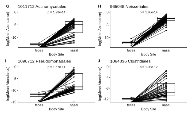
The general trend observed with most of these top nasal taxa is that most patients have very low abundance of these taxa in the feces. This is especially apparent in Figure 4.3.3 plots D, G, and F, in which most lines begin very low in the feces and rise in the nasal cavity. As observed previously within the top fecal taxa, there is also an OTU within these top nasal taxa (Figure 4.3.3.C, 1059772 Bacillales) that has greater abundance in the feces than in the nasal cavity. When a two-sided paired Wilcoxon rank-sum test was performed for this OTU, a statistically significant difference was found between the two groups (p « 0.05), indicating that the abundance of this OTU is significantly greater in the feces.
5 - Discussion
The results of these analyses revealed much about the different microbiomes during the onset of diabetes. Based on both alpha and beta diversity measures, the fecal and nasal microbiomes are significantly different, both in terms of the amount of diversity and the dominating taxa present. Both alpha diversity measures computed (species richness and Shannon diversity) reveal that the fecal microbiome of these pre-diabetic patients is significantly more diverse than the nasal microbiome, with a wider range of bacteria (Figures 4.1.1 and 4.1.2). This is in support of Hypothesis #1.
Furthermore, the PERMANOVA test reveals that the two microbiomes are significantly different from each other, in support of Hypothesis #2. However, when looking at the most abundant taxa of the two body sites, there appears to be more diversity in the nasal microbiome than the fecal one (Figure 4.2.1). There is also an emergence of patterns as more samples are included in the analysis. We see that the fecal samples appear to group together and display similarity when compared to the nasal samples that disperse as the analysis parameters become less restrictive. Overall, the analysis using the most abundant taxa found that the nasal cavity nurtures a more diverse microbiome, but the alpha diversity measure found the opposite when looking at all samples from both body sites. It can be inferred that this is due to the many taxa present in small quantities in the feces. This is consistent with the findings of other studies that declare the fecal microbiome is diverse, but dominated by a few taxa (Lozupone et al, 2012).
The top 20 taxa that we identified appear to be driving the differences between the two body sites. 18 out of 20 of the top taxa were found to be significantly higher in the body site they were identified with, suggesting that these taxa are among the defining taxa that distinguish the two microbial communities. Bacteroidales was the dominating Order in the feces and Actinomycetales was the dominating Order in the nasal cavity, both of which are reported in literature to be among the highest abundant bacteria in their respective body sites in healthy patients (Mestecky, 2015; Piquer-Esteban et al, 2021).
In the context of Type II diabetes, Bacteroidales in the feces is reported to be negatively associated with the disease (Gurung et al, 2020). This is contradictory to our findings, as we found that Bacteroidales is still highly abundant in these pre-diabetic patients. However, it is important to note that our patients are pre-diabetic and it is uncertain whether or not their microbiomes have been impacted by the onset of this disease. It would not be possible to determine this without healthy patients acting as a control group.
5.1 Further Directions
In order to more clearly determine the relationship between nasal and fecal microbiomes and type 2 diabetes, more data is required. It would be helpful to have data from healthy patients to be used as a control group and data from patients with type 2 diabetes would also be of great interest for comparison. For example, it is possible that Bacteroidales have a much less significant presence in the pre-diabetic patients used in this study than is normal for healthy patients, which would be consistent with the conjecture that Bacteroidales is negatively associated with the disease (Gurung et al, 2020). It has also been found that the diversity of the microbiomes are significantly associated with diabetes onset age (Krych et al, 2015). It is important to note that patient ages were not available to us in this study, so age could be a confounding factor that affects our results and would be a valuable variable for future study. In another case, there has been some recent evidence that a diverse fecal microbiome is an indicator of good health, highlighting the importance of comparing microbial groups at various stages of disease progression (healthy, pre-diabetic, and diabetic) to better understand the progression of type 2 diabetes (Khan et al, 2021). This project has been a starting point to doing so.
6 - References
Caporaso, J.G., Kuczynski J., Stombaugh J. et al. QIIME allows analysis of high-throughput community sequencing data. Nat. Methods 7, 335–336 (2010).
Gurung, M., Li, Z., You, H. et al. Role of gut microbiota in type 2 diabetes pathophysiology. EBioMedicine 51(102590) (2020). https://doi.org/10.1016/j.ebiom.2019.11.051.
Integrated Personal Omics Profiling. Stanford Medicine, https://med.stanford.edu/ipop.html
Khan N, Lindner S, Gomes ALC, Devlin SM, Shah GL, Sung AD, Sauter CS, Landau HJ, Dahi PB, Perales MA, Chung DJ, Lesokhin AM, Dai A, Clurman A, Slingerland JB, Slingerland AE, Brereton DG, Giardina PA, Maloy M, Armijo GK, Rondon-Clavo C, Fontana E, Bohannon L, Ramalingam S, Bush AT, Lew MV, Messina JA, Littmann E, Taur Y, Jenq RR, Chao NJ, Giralt S, Markey KA, Pamer EG, van den Brink MRM, Peled JU. Fecal microbiota diversity disruption and clinical outcomes after auto-HCT: a multicenter observational study. Blood. 2021 Mar 18;137(11):1527-1537. doi: 10.1182/blood.2020006923. PMID: 33512409; PMCID: PMC7976512.
Krych Ł, Nielsen DS, Hansen AK, Hansen CH. Gut microbial markers are associated with diabetes onset, regulatory imbalance, and IFN-γ level in NOD mice. Gut Microbes. 2015;6(2):101-9. doi: 10.1080/19490976.2015.1011876. Epub 2015 Feb 3. PMID: 25648687; PMCID: PMC4615729.
Lozupone CA, Stombaugh JI, Gordon JI, Jansson JK, Knight R. Diversity, stability and resilience of the human gut microbiota. Nature. 2012 Sep 13;489(7415):220-30. doi: 10.1038/nature11550. PMID: 22972295; PMCID: PMC3577372.
Maruthur, Nisa Marisa. “Prediabetes.” www.hopkinsmedicine.org, 16 Feb. 2023, www.hopkinsmedicine.org/health/conditions-and-diseases/diabetes/prediabetes.
Mestecky, J. (2015). Mucosal immunology. Academic Press.
Piquer-Esteban S., Ruiz-Ruiz S., Arnau V. et al. Exploring the universal healthy human gut microbiota around the World. Comput Struct Biotechnol J. 20:421-433. (2021). https://doi.org/10.1016/j.csbj.2021.12.035.
Zhou, W., Sailani, M.R., Contrepois, K. et al. Longitudinal multi-omics of host–microbe dynamics in prediabetes. Nature 569, 663–671 (2019). https://doi.org/10.1038/s41586-019-1236-x.